Lightness And Darkness In Art

Property of a color

Three hues in the Munsell color model. Each colour differs in value from acme to bottom in equal perception steps. The correct column undergoes a dramatic change in perceived color.

Lightness is a visual perception of the luminance ${\displaystyle (L)}$ of an object. It is frequently judged relative to a similarly lit object. In colorimetry and color appearance models, lightness is a prediction of how an illuminated color will announced to a standard observer. While luminance is a linear measurement of light, lightness is a linear prediction of the human perception of that light.

This is considering human vision's lightness perception is not-linear relative to light. Doubling the quantity of light does not issue in a doubling in perceived lightness, simply a modest increment.

The symbol for perceptual lightness is unremarkably either ${\displaystyle J}$ as used in CIECAM02 or ${\displaystyle L^{*}}$ every bit used in CIELAB and CIELUV. ${\displaystyle L^{*}}$ ("Lstar") is not to exist confused with ${\displaystyle L}$ as used for luminance. In some color ordering systems such as Munsell, Lightness is referenced as value.

Chiaroscuro and Tenebrism both take advantage of dramatic contrasts of value to raise drama in art. Artists may also employ shading, subtle manipulation of value.

Lightness in dissimilar colorspaces [edit]

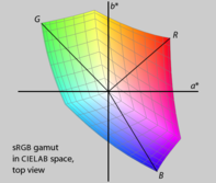
Fig 2a. The sRGB gamut mapped in CIELAB infinite. Find that the lines pointing to the crimson, light-green, and blue primaries are not evenly spaced by hue angle, and are of unequal length. The primaries also have dissimilar L* values.

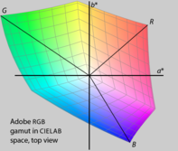
Fig 2b. The Adobe RGB gamut mapped in CIELAB space. Also observe that these two RGB spaces have different gamuts, and thus volition have different HSL and HSV representations.

In some colorspaces or colour systems such as Munsell, HCL, and CIELAB, the lightness (value) achromatically constrains the maximum and minimum limits, and operates independently of the hue and chroma. For instance Munsell value 0 is pure black, and value 10 is pure white. Colors with a discernible hue must therefore have values in betwixt these extremes.

In a subtractive color model (east.g. pigment, dye, or ink) lightness changes to a color through various tints, shades, or tones can be achieved by calculation white, black, or grayness respectively. This also reduces saturation.

In HSL and HSV, the displayed luminance is relative to the hue and chroma for a given lightness value, in other words the selected lightness value does not predict the actual displayed luminance nor the perception thereof. Both systems utilise coordinate triples, where many triples can map onto the same color.

In HSV, all triples with value 0 are pure black. If the hue and saturation are held constant, then increasing the value increases the luminance, such that a value of one is the lightest color with the given hue and saturation. HSL is similar, except that all triples with lightness 1 are pure white. In both models, all pure saturated colors indicate the same lightness or value, merely this does not relate to the displayed luminance which is determined by the hue. I.e. xanthous is higher luminance than blue, fifty-fifty if the lightness value is set at a given number.

While HSL, HSV, and like spaces serve well enough to choose or adjust a single color, they are not perceptually uniform. They trade off accuracy for computational simplicity, as they were created in an era where computer technology was restricted in operation. ^[ane]

If we take an image and extract the hue, saturation, and lightness or value components for a given color space, we will see that they may differ substantially from a unlike colour infinite or model. For case, examine the following images of a burn breather (fig. 1). The original is in the sRGB color space. CIELAB ${\displaystyle Fifty^{*}}$ is a perceptually uniform lightness prediction that is derived from luminance ${\displaystyle Y}$ , only discards the ${\displaystyle X}$ and ${\displaystyle Z}$ , of the CIE XYZ color space. Notice this appears similar in perceived lightness to the original colour epitome. Luma ${\displaystyle (Y^{\prime number })}$ is a gamma-encoded luminance component of some video encoding systems such equally ${\displaystyle (Y^{\prime }IQ)}$ and ${\displaystyle (Y^{\prime }UV)}$ . It is roughly similar, merely differs at loftier blush, diffusive almost from an achromatic indicate such as linear luminance ${\displaystyle Y}$ or not-linear lightness ${\displaystyle L^{*}}$ . HSL ${\displaystyle L}$ and HSV ${\displaystyle V}$ are neither perceptually compatible, nor compatible as to luminance.

Fig. 1a. Colour photograph (sRGB color space).

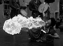
Fig. 1b. CIELAB L* (further transformed dorsum to sRGB for consistent display).

Fig. 1c. Rec. 601 luma Y′.

Fig. 1d. Component average: "intensity" I.

Fig. 1e. HSV value V.

Fig. 1f. HSL lightness L.

Relationship to value and relative luminance [edit]

The Munsell value has long been used every bit a perceptually compatible lightness calibration. A question of interest is the relationship between the Munsell value scale and the relative luminance. Aware of the Weber–Fechner law, Albert Munsell remarked "Should we utilize a logarithmic bend or bend of squares?"^[2] Neither choice turned out to be quite correct; scientists eventually converged on a roughly cube-root curve, consequent with the Stevens'due south ability law for brightness perception, reflecting the fact that lightness is proportional to the number of nerve impulses per nerve fiber per unit fourth dimension.^[3] The residuum of this section is a chronology of lightness models, leading to CIECAM02.

Note. – Munsell's Five runs from 0 to 10, while Y typically runs from 0 to 100 (often interpreted equally a percentage). Typically, the relative luminance is normalized so that the "reference white" (say, magnesium oxide) has a tristimulus value of Y = 100. Since the reflectance of magnesium oxide (MgO) relative to the perfect reflecting diffuser is 97.5%, Five = 10 corresponds to Y = 100 / 97.5 % ≈ 102.6 if MgO is used as the reference.^[iv]

Observe that the lightness is 50% for a relative luminance of around 18% relative to the reference white.

1920 [edit]

Irwin Priest, Kasson Gibson, and Harry McNicholas provide a bones estimate of the Munsell value (with Y running from 0 to ane in this case):^[5]

${\displaystyle V=10{\sqrt {Y}}.}$

1933 [edit]

Alexander Munsell, Louise Sloan, and Isaac Godlove launch a study on the Munsell neutral value calibration, because several proposals relating the relative luminance to the Munsell value, and suggest:^{[half dozen] [seven]}

${\displaystyle V^{two}=1.4742Y-0.004743Y^{2}.}$

1943 [edit]

Sidney Newhall, Dorothy Nickerson, and Deane Judd gear up a written report for the Optical Society of America (OSA) on Munsell renotation. They propose a quintic parabola (relating the reflectance in terms of the value):^[8]

${\displaystyle Y=i.2219V-0.23111V^{2}+0.23951V^{3}-0.021009V^{iv}+0.0008404V^{five}.}$

1943 [edit]

Using Tabular array Ii of the OSA written report, Parry Moon and Domina Spencer express the value in terms of the relative luminance:^[9]

${\displaystyle V=v\left({\frac {Y}{19.77}}\correct)^{0.426}=1.4Y^{0.426}.}$

1944 [edit]

Jason Saunderson and B.I. Milner introduce a subtractive constant in the previous expression, for a better fit to the Munsell value.^[10] Later, Dorothea Jameson and Leo Hurvich merits that this corrects for simultaneous contrast effects.^{[eleven] [12]}

${\displaystyle Five=2.357Y^{0.343}-i.52.}$

1955 [edit]

Ladd and Pinney of Eastman Kodak are interested in the Munsell value as a perceptually uniform lightness scale for use in television. Afterwards because one logarithmic and v power-law functions (per Stevens' power law), they relate value to reflectance by raising the reflectance to the power of 0.352:^[13]

${\displaystyle Five=2.217Y^{0.352}-1.324.}$

Realizing this is quite close to the cube root, they simplify it to:

${\displaystyle V=ii.468{\sqrt[{iii}]{Y}}-1.636.}$

1958 [edit]

Glasser et al. define the lightness as ten times the Munsell value (so that the lightness ranges from 0 to 100):^[xiv]

${\displaystyle L^{\star }=25.29{\sqrt[{3}]{Y}}-18.38.}$

1964 [edit]

Günter Wyszecki simplifies this to:^[15]

${\displaystyle West^{\star }=25{\sqrt[{3}]{Y}}-17.}$

This formula approximates the Munsell value office for 1% < Y < 98% (information technology is non applicative for Y < 1%) and is used for the CIE 1964 colour space.

1976 [edit]

CIELAB uses the following formula:

${\displaystyle L^{\star }=116\left({\frac {Y}{Y_{\mathrm {n} }}}\right)^{\frac {1}{iii}}-16.}$

where Y _n is the CIE XYZ Y tristimulus value of the reference white point (the subscript n suggests "normalized") and is discipline to the brake Y / Y _northward > 0.01. Pauli removes this restriction by computing a linear extrapolation which maps Y / Y _north = 0 to 50* = 0 and is tangent to the formula above at the point at which the linear extension takes effect. Get-go, the transition bespeak is determined to be Y / Y _n = ( 6 / 29 )³ ≈ 0.008856, then the gradient of ( 29 / 3 )ⁱⁱⁱ ≈ 903.3 is computed. This gives the two-office function:^[16]

${\displaystyle f(t)={\begin{cases}t^{\frac {ane}{3}}&{\text{if }}t>\left({\frac {6}{29}}\right)^{3}\\{\frac {1}{3}}\left({\frac {29}{6}}\right)^{2}t+{\frac {iv}{29}}&{\text{otherwise}}\finish{cases}}}$

The lightness is then:

${\displaystyle L^{\star }=116f\left({\frac {Y}{Y_{\mathrm {northward} }}}\right)-16.}$

At first glance, you lot might approximate the lightness function by a cube root, an approximation that is found in much of the technical literature. Notwithstanding, the linear segment well-nigh black is meaning, so the 116 and 16 coefficients. The all-time-fit pure power function has an exponent of about 0.42, far from 1 / 3 .^[17] An approximately 18% grey card, having an exact reflectance of ( 33 / 58 )³, has a lightness value of fifty. It is called "mid greyness" considering its lightness is midway between blackness and white.

1997 [edit]

As early as in 1967 a hyperbolic relationship between light intensity and cone jail cell responses was discovered in fish, in line with the Michaelis–Menten kinetics model of biochemical reactions.^[18] In the 70s the same relationship was found in a number of other vertebrates and in 1982, using microelectrodes to measure out cone responses in living rhesus macaques, Valeton and Van Norren constitute the following relationship:^[19]

1 / V ~ 1 + (σ / I)^0.74

where 5 is the measured potential, I the light intensity and σ a constant. In 1986 Seim and Valberg realised that this relationship might aid in the structure of a more than uniform colour space.^[20] This inspired advances in color modelling and when the International Commission on Illumination held a symposium in 1996, objectives for a new standard colour model were formulated and in 1997 CIECAM97s (International Commission on Illumination, colour appearance model, 1997, simple version) was standardised.^[21] CIECAM97s distinguishes between lightness, how lite something appears compared to a similarly lit white object, and effulgence, how much lite appears to shine from something.^[22] According to CIECAM97s the lightness of a sample is:

J = 100 (A_sample / A_white)^cz

In this formula, for a small sample under brilliant weather in a surrounding field with a relative luminance n compared to white, c has been called such that:

${\displaystyle {\text{cz}}={\frac {1+{\sqrt {north}}}{ane+{\sqrt {\frac {1}{5}}}}}}$

This models that a sample will appear darker on a light groundwork than on a dark background. Run into contrast outcome for more information on the topic. When due north = 1 / 5 , cz = one, representing the supposition that almost scenes accept an average relative luminance of 1 / 5 compared to bright white, and that therefore a sample in such a environs should be perceived at its proper lightness. The quantity A models the achromatic cone response; it is color dependent but for a gray sample under bright weather it works out as:

${\displaystyle {\frac {\text{A}}{{\text{North}}_{\text{bb}}}}={\frac {122}{ane+2{\Bigl (}{\tfrac {1}{x}}Y{\sqrt[{iii}]{5L_{A}}}{\Bigr )}^{-0.73}}}+1}$

N_bb is a fudge cistron that is normally ane; it's only of concern when comparing effulgence judgements based on slightly different reference whites.

Hither Y is the relative luminance compared to white on a scale of 0 to 1 and L_A is the average luminance of the adapting visual field every bit a whole, measured in cd/thousand². The achromatic response follows a kind of S-curve, ranging from one to 123, numbers which follow from the manner the cone responses are averaged and which are ultimately based on a crude estimate for the useful range of nerve impulses per second, and which has a fairly large intermediate range where it roughly follows a square root curve. The effulgence according to CIECAM97s is then:

Q = (1.24 / c) (J / 100)^0.67 (A_white + 3)^0.9

The factor 1.24 / c is a environs gene that reflects that scenes appear brighter in dark surrounding weather. Suggestions for a more than comprehensive model, CIECAM97C, were too formulated, to take into account several furnishings at extremely dark or bright weather condition, coloured lighting, besides equally the Helmholtz–Kohlrausch consequence, where highly chromatic samples appear lighter and brighter in comparing to a neutral grey. To model the latter consequence, in CIECAM97C the formula for J is adjusted as follows:

J_HK = J + (100 – J) (C / 300) |sin(½h – 45°)|,

where C is the chroma and h the hue bending

Q is and so calculated from J_HK instead of from J. This formula has the effect of pulling up the lightness and effulgence of coloured samples. The larger the blush, the stronger the upshot; for very saturated colours C tin be close to 100 or even higher. The absolute sine term has a abrupt V-shaped valley with a nil at yellow and a broad plateau in the deep blues.^[23]

2002 [edit]

The achromatic response in CIECAM97s is a weighted addition of cone responses minus 2.05. Since the total dissonance term adds up to 3.05, this ways that A and consequentially J and Q aren't nix for accented black. To set up this, Li, Luo & Hunt suggested subtracting 3.05 instead, and so the scale starts at zero.^[24] Although CIECAM97s was a successful model to spur and direct colorimetric research, Fairchild felt that for applied applications some changes were necessary. Those relevant for lightness calculations were to, rather than apply several discrete values for the surroundings factor c, allow for linear interpolation of c and thereby allowing the model to be used under intermediate surround conditions, and to simplify z to remove the special instance for large stimuli because he felt it was irrelevant for imaging applications.^[25] Based on experimental results, Hunt, Li, Juan and Luo proposed a number of improvements. Relevant for the topic at mitt is that they suggested lowering z slightly.^[26] Li and Luo found that a colour space based on such a modified CIECAM97s using lightness as one of the coordinates was more perceptually uniform than CIELAB.^[27] Because of the shape of the cone response S-curve, when the luminance of a colour is reduced, even if its spectral composition remains the same, the different cone responses don't quite change at the same rate with respect to each other. Information technology is plausible therefore that the perceived hue and saturation volition change at low luminance levels. Simply CIECAM97s predicts much larger deviations than are by and large thought probable and therefore Hunt, Li and Luo suggested using a cone response curve which approximates a ability curve for a much larger range of stimuli, so hue and saturation are better preserved.^[28] All these proposals, every bit well every bit others relating to chromaticity, resulted in a new colour advent model, CIECAM02. In this model, the formula for lightness remains the aforementioned:

J = 100 (A_sample / A_white)^cz

But all the quantities that feed into this formula change in some manner. The parameter c is now continuously variable as discussed above and z = ane.48 + √north. Although this is higher than z in CIECAM97s, the total constructive power factor is very similar considering the effective power factor of the achromatic response is much lower:

${\displaystyle {\frac {\text{A}}{{\text{N}}_{\text{bb}}}}={\frac {1220}{1+{\frac {27.13}{\left({\frac {{\sqrt[{3}]{v{\text{Fifty}}_{\text{A}}}}{\text{Y}}}{ten}}\right)^{0.42}}}}}}$

As earlier, this formula assumes bright weather. Apart from 1220, which results from an arbitrarily assumed cone response constant, the various constants in CIECAM02 were fitted to experimental data sets. The expression for the brightness has as well changed considerably:

${\displaystyle Q={\frac {iv}{c}}{\frac {\sqrt {J}}{10}}(A_{white}+4)\left({\frac {\sqrt[{3}]{5L_{A}}}{10}}\right)^{0.25}}$

Note that contrary to the suggestion from CIECAM97C, CIECAM02 contains no provision for the Helmholtz–Kohlrausch effect.^{[29] [30]}

Other psychological effects [edit]

This subjective perception of luminance in a non-linear fashion is one thing that makes gamma pinch of images worthwhile. Abreast this miracle there are other effects involving perception of lightness. Chromaticity can bear on perceived lightness as described by the Helmholtz–Kohlrausch effect. Though the CIELAB space and relatives do non account for this effect on lightness, it may be implied in the Munsell colour model. Lite levels may also affect perceived chromaticity, equally with the Purkinje consequence.

Encounter also [edit]

• Brightness
• Tint, shade and tone

Notes [edit]

References [edit]

1. ^ Almost of the disadvantages below are listed in A Technical Introduction to Digital Video (1996) by Charles Poynton, though as mere statements, without examples.
2. ^ Kuehni, Rolf G. (February 2002). "The early on evolution of the Munsell system". Colour Research & Application. 27 (1): 20–27. doi:10.1002/col.10002.
3. ^ Hunt, Robert Westward. G. (May 18, 1957). "Light Energy and Brightness Sensation". Nature. 179 (4568): 1026. doi:ten.1038/1791026a0. PMID 13430776.
4. ^ Valberg, Arne (2006). Light Vision Colour. John Wiley and Sons. p. 200. ISBN978-0470849026.
5. ^ Priest, Irwin G.; Gibson, One thousand.S.; McNicholas, H.J. (September 1920). "An examination of the Munsell color arrangement. I: Spectral and total reflection and the Munsell scale of Value". Technical newspaper 167 (3). Usa Bureau of Standards: 27.
6. ^ Munsell, A.Due east.O.; Sloan, 50.L.; Godlove, I.H. (November 1933). "Neutral value scales. I. Munsell neutral value scale". JOSA. 23 (11): 394–411. doi:10.1364/JOSA.23.000394. Note: This paper contains a historical survey stretching to 1760.
7. ^ Munsell, A.E.O.; Sloan, L.L.; Godlove, I.H. (Dec 1933). "Neutral value scales. 2. A comparison of results and equations describing value scales". JOSA. 23 (12): 419–425. doi:10.1364/JOSA.23.000419.
8. ^ Newhall, Sidney M.; Nickerson, Dorothy; Judd, Deane B (May 1943). "Terminal report of the O.Southward.A. subcommittee on the spacing of the Munsell colors". Journal of the Optical Society of America. 33 (7): 385–418. doi:x.1364/JOSA.33.000385.
9. ^ Moon, Parry; Spencer, Domina Eberle (May 1943). "Metric based on the composite color stimulus". JOSA. 33 (5): 270–277. doi:10.1364/JOSA.33.000270.
10. ^ Saunderson, Jason L.; Milner, B.I. (March 1944). "Further study of ω space". JOSA. 34 (3): 167–173. doi:10.1364/JOSA.34.000167.
11. ^ Hurvich, Leo Grand.; Jameson, Dorothea (November 1957). "An Opponent-Process Theory of Color Vision". Psychological Review. 64 (vi): 384–404. doi:x.1037/h0041403. PMID 13505974.
12. ^ Jameson, Dorothea; Leo M. Hurvich (May 1964). "Theory of effulgence and color contrast in human vision". Vision Research. four (1–2): 135–154. doi:10.1016/0042-6989(64)90037-9. PMID 5888593.
13. ^ Ladd, J.H.; Pinney, J.E. (September 1955). "Empirical relationships with the Munsell Value calibration". Proceedings of the Institute of Radio Engineers. 43 (9): 1137. doi:10.1109/JRPROC.1955.277892.
14. ^ Glasser, L.Chiliad.; A.H. McKinney; C.D. Reilly; P.D. Schnelle (October 1958). "Cube-root color coordinate arrangement". JOSA. 48 (10): 736–740. doi:10.1364/JOSA.48.000736.
15. ^ Wyszecki, Günter (November 1963). "Proposal for a New Color-Deviation Formula". JOSA. 53 (11): 1318–1319. doi:x.1364/JOSA.53.001318. Note: The asterisks are not used in the paper.
16. ^ Pauli, Hartmut Grand.A. (1976). "Proposed extension of the CIE recommendation on "Uniform color spaces, color spaces, and color-difference equations, and metric color terms"". JOSA. 66 (8): 866–867. doi:ten.1364/JOSA.66.000866.
17. ^ Poynton, Charles; Funt, Brian (February 2014). "Perceptual uniformity in digital image representation and display". Color Research and Awarding. 39 (1): 6–fifteen. doi:10.1002/col.21768.
18. ^ Ken-Ichi Naka & William Albert Hugh Rushton: The generation and spread of S-potentials in fish (Cyprinidae)
19. ^ Jean Mathieu Valeton & Dirk van Norren: Calorie-free adaptation of primate cones: An analysis based on extracellular data
20. ^ Thorstein Seim & Arne Valberg: Towards a uniform color space: A amend formula to depict the Munsell and OSA color scales
21. ^ Mark D. Fairchild: Colour Advent Models § The CIE Color Appearance Model (1997), CIECAM97s
22. ^ Robert William Gainer Chase: Some comments on using the CIECAM97s colour-appearance model
23. ^ Ming Ronnier Luo & Robert William Gainer Hunt: The structure of the CIE 1997 colour appearance model
24. ^ Changjun Li, Ming Ronnier Luo & Robert William Gainer Hunt: A revision of the CIECAM97s model
25. ^ Mark D. Fairchild: A revision of CIECAM97s for practical applications
26. ^ Robert William Gainer Hunt, Changjun Li, Lu-Yin Grace Juan & Ming Ronnier Luo: Farther improvements to CIECAM97s (also cited every bit Further refinements to CIECAM97s)
27. ^ Changjun Li & Ming Ronnier Luo: A compatible colour space based upon CIECAM97s
28. ^ Robert William Gainer Hunt, Changjun Li & Ming Ronnier Luo: Dynamic cone response functions for models of colour appearance
29. ^ Nathan Moroney, Mark D. Fairchild, Robert William Gainer Chase, Changjun Li, Ming Ronnier Luo & Todd Newman: The CIECAM02 color appearance model
30. ^ CIE technical committee: Color Advent Models for Colour Management Applications

External links [edit]

Media related to Lightness at Wikimedia Commons

Lightness And Darkness In Art,

Source: https://en.wikipedia.org/wiki/Lightness

Posted by: edwardsloges1978.blogspot.com

Share this post